Back to the list

Opinion

Developing a Novel Solution for Measuring Weight - Part 4

Published on 01 Feb, 2024 by Neil

First Full Characterisation

The Python application which was used to collect the temperature coefficient measurements was modified so that the displacement values read from the micrometer head could be entered manually and then the frequency, temperature and humidity measurements were all taken automatically. This works out well, but the step size was small (0.05mm) and many measurements were taken. After the data is accrued in the Influx database, the records can be extracted and processed.

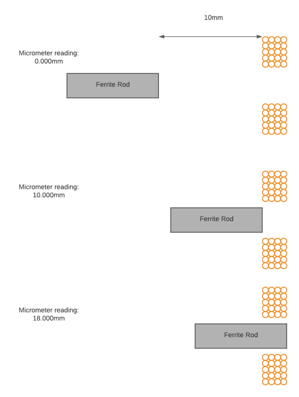
The micrometer head was wound to a position 10mm from the start of the inductor-former. This micrometer was then reset to zero and this acts as a datum for all the measurements. The diagram below shows this (the inductor is on the right, shown by sections of copper turns):

Full Range Results

A total of 360 measurements were taken in 0.05mm steps over a displacement of 18.0mm. This is plotted below:

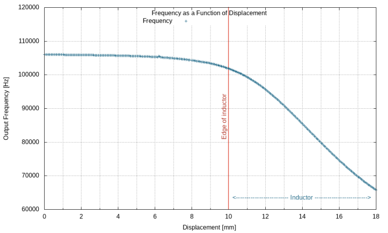
The design criteria for the displacement sensor is that the full scale (0 to 1kg) is achieved with a 5mm displacement. The region with good linearity can be seen from 11mm to 16mm. As the displacement will need to be interpolated from a table of calibration values, good linearity means fewer points in the calibration table.

A plot of the region from 11mm to 16mm with a linear trend line is shown below:

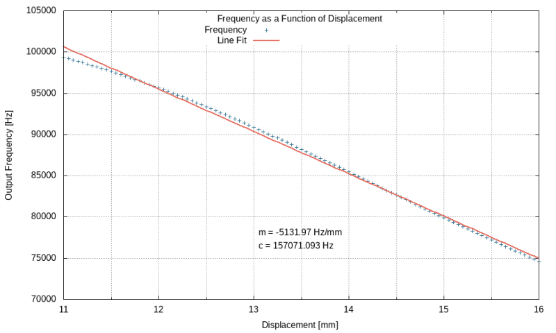
The gradient of the line (m) is -5132Hz/mm or 5.13Hz/μm! This is very good as the output is stable to ~2 decimals and this swing can be easily measured to a high degree of accuracy. The temperature coefficient was found to be 9.4Hz/°C so the approximate drift due to temperature can now be calculated.

Predicted Temperature Effects

A temperature-controlled environmental chamber is not available so the only option is to calculate the drift of measured weight based on the temperature coefficient determined previously.

To interpret the table, consider that all measured masses should be 30g. However, the frequency changes as a function of temperature so the table shows a range of reported masses due to the temperature variation. The operating temperature range is 10 to 30°C. The reference frequency and temperature is 98867.7721Hz at 25°C. Calculations of the frequency as a function of temperature are determined from this reference. The tempco. used is 9.3941Hz/°C. The mass is the predicted reading at the temperature of that row and ideally would be 30g corresponding to a displacement of 0.15mm.

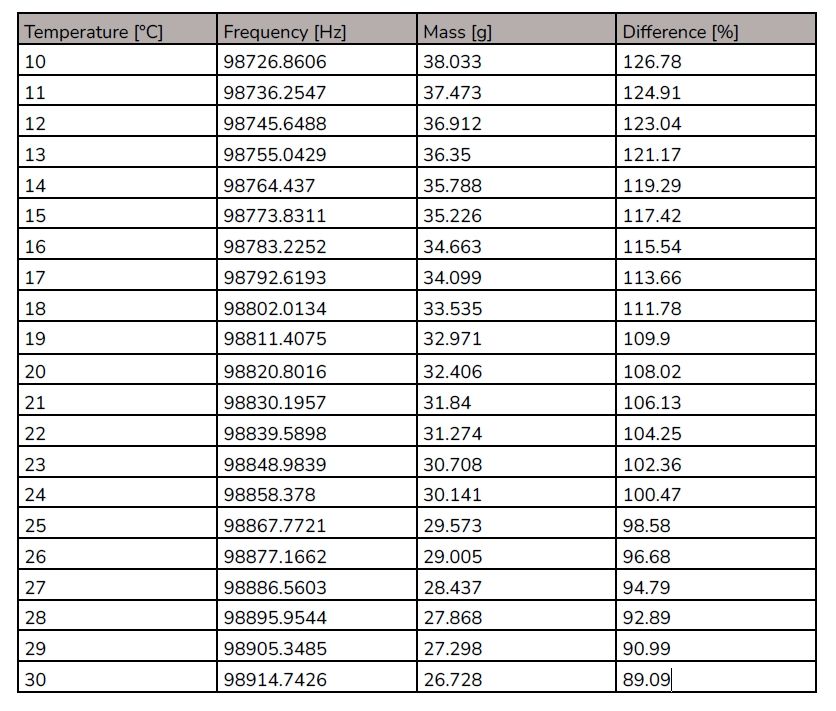
These results are interpolated using the Lagrange method (described later). Unsurprisingly, the measured weight is most accurate around the reference temperature of 25°C.

At 10°C the drift is 8g over and at 30°C the measurement is 3.3g under. It is not clear whether this is good enough or if temperature compensation will need to be applied.

Interpolation

The points between 11 and 16mm are reasonably linear and will form the operating region for the displacement sensor. The next task is to find a computationally low-cost method to interpolate between calibration points and then check that the calculated value is within the tolerance required.

The diagram below helps to introduce the concept:

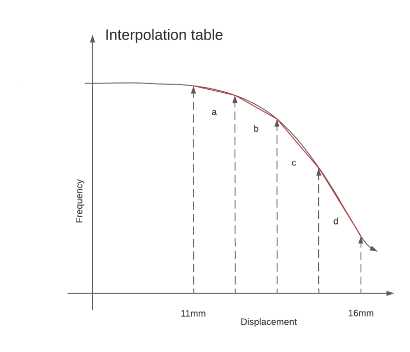
This diagram represents the principle, that the linearity of the data collected from the displacement sensor is much better than this example. We have four segments a, b,c and d, and a line in red which joins the points together. The vertical arrow-headed lines represent the calibration points when the displacement sensor is extended by a calibration weight, for example. Each line segment (a to d) has a gradient and intercept represented by the general form:

F = mx + c

If a frequency measurement is made which lies between the calibration points, an algorithm can be used to find an approximation for the displacement which generated that frequency. As can be seen in segments b and c, there is a gap between the red line and the actual frequency. This will produce an error in the weight of the object being measured in the final application. One method to reduce this systematic error is to reduce the segment length by having more entries in the calibration table. This then pushes the problem back to the end-of-line calibrator, the calibration becomes slow and laborious with an impact on the resources of the micro controller required to store the calibration values.

The Python code to perform the linear interpolation is below:

DISP = 0
FREQ = 1
# Displacement, frequency
calibration_table = [
[ 11.0, 99346.1514 ],
[ 12.0, 95649.5188 ],
[ 13.0, 90867.9063 ],
[ 14.0, 85448.4024 ],
[ 15.0, 79887.5105 ],
[ 16.0, 74595.7611 ]
]

class Segment:
def __init__(self, d0 = 0.0, d1 = 0.0, f0 = 0.0, f1 = 0.0):
“”” Create a new segment “””
self.d0 = d0
self.d1 = d1
self.f0 = f0
self.f1 = f1

def getDisplacementSpan(self):
# Determine the displacement span for this segment.
return self.d1 - self.d0

def getFrequencySpan(self):
# Determine the frequency span for this segment.
return self.f0 - self.f1

def interpolate_segment(segment, frequency):
	
# Initialise as a fail.
result = 0

d_span = segment.getDisplacementSpan()
f_span = segment.getFrequencySpan()

# Final check that we can interpolate this segment.
if (frequency <= segment.f0 and frequency >= segment.f1):

# Do the multiply before the divide to avoid rounding errors.
result = segment.d0 + (((segment.f0 - frequency) * d_span) / f_span)
return result

def interpolate_table(frequency):
displacement = 0
if (frequency >= calibration_table[-1][FREQ]) and \
(frequency <= calibration_table[0][FREQ]):

# Iterate the table length less one.
loop_len = len(calibration_table) - 1

# Find the segment that this frequency belongs to.
for index in range(loop_len):

# Get the adjacent elements in the look up table.
first = calibration_table[index]
second = calibration_table[index + 1]

# Check the range to see if the frequency of interest lies within this segment.
if (first[FREQ] > frequency and second[FREQ] < frequency):

# Create a segment object and interpolate on this segment.
segment = Segment(first[DISP], second[DISP], first[FREQ],
second[FREQ])
displacement = interpolate_segment(segment, frequency)
return displacement

This code was derived from C and can be easily ported to a microcontroller.

Linear Interpolation Results

Each segment starts and finishes on a calibration sample point. Therefore the worst-case value (to maximise the error) is at the midpoints of the segment. With this in mind, the table below shows the errors. Note that in the final application, a 1mm displacement will equate to 200g.

# Test data used.
test_table = [
# Actual, Input
[ 11.50, 97650.2112 ],
[ 12.50, 93376.509 ],
[ 13.50, 88204.6578 ],
[ 14.50, 82660.8346 ],
[ 15.50, 77187.6638 ],
]

expected: 100.000g, actual 91.756g, difference 91.76%
expected: 300.000g, actual 295.073g, difference 98.36%
expected: 500.000g, actual 498.284g, difference 99.66%
expected: 700.000g, actual 700.256g, difference 100.04%
expected: 900.000g, actual 902.040g, difference 100.23%

The results for 500g, 700g and 900g are very good. The results at 300g are acceptable, but the 100g (which is above the weight where the vessel detect operates) is poor. This is because the segment between 11mm and 12mm has a higher gradient than the rest of the curve. An alternative interpolation method is required.

Lagrange Interpolation

Another interpolation technique available is Lagrange Interpolation. This fits a polynomial between the segments rather than a linear fit. The advantage will be seen where the curve deviates from being linear.

A Python implementation for the Lagrange interpolation method is below:


# Calibration table length
n = 6

y = [ 11.0, 12.0, 13.0, 14.0, 15.0, 16.0 ]
x = [ 99346.1514, 95649.5188, 90867.9063, 85448.4024, 79887.5105, 74595.7611
]

def interpolate(xp):
# Set interpolated value initially to zero
yp = 0

# Implementing Lagrange Interpolation
for i in range(n):
p = 1
for j in range(n):
if i != j:
p = p * (xp - x[j])/(x[i] - x[j])
yp = yp + p * y[i]
return yp

Running this interpolation method on the same test data used above yields the following results:

python3 lagrange.py
expected: 100.000g, actual 99.273g, difference 99.27%
expected: 300.000g, actual 300.083g, difference 100.03%
expected: 500.000g, actual 499.788g, difference 99.96%
expected: 700.000g, actual 700.182g, difference 100.03%
expected: 900.000g, actual 899.245g, difference 99.92%

As expected, the results where the curve is nonlinear are much improved.

Repeatability

The final application has to provide repeatable results. The next investigation was to see if the frequency was a factor of the direction of insertion and if the same frequency could be achieved each time. The calibration values were taken from cold:

y = [ 11.0, 12.0, 13.0, 14.0, 15.0, 16.0 ]
x = [ 99441.5707, 95781.6696, 91018.5973, 85594.1532, 80039.4454, 74735.0054]

The ferrite was wound out to 9mm, and then to 11.25mm, 13.5mm and 15.75mm. Then the ferrite was wound to 17mm and back to 15.75mm, 13.5mm and 11.25mm. Finally, the ferrite is wound out to 9mm and the whole process is repeated thirteen times. The results tables below are in ascending order of frequency.

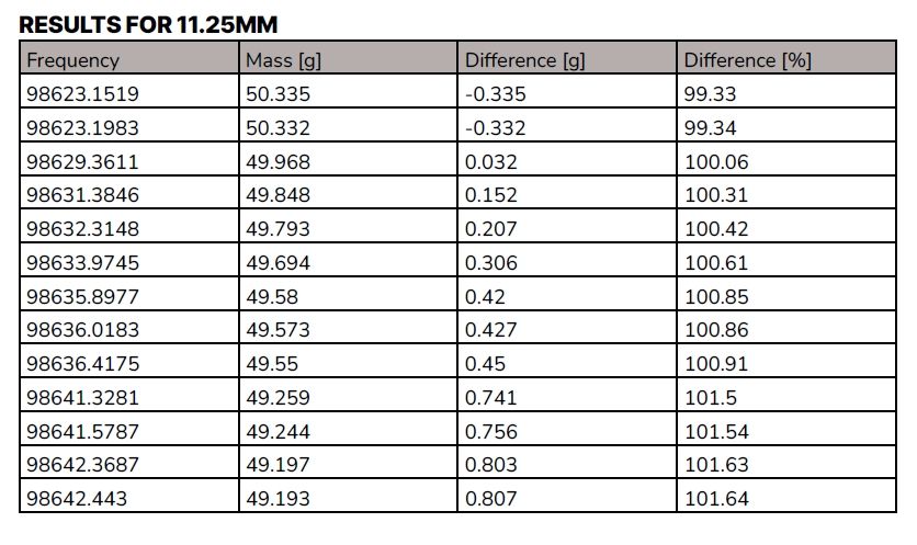
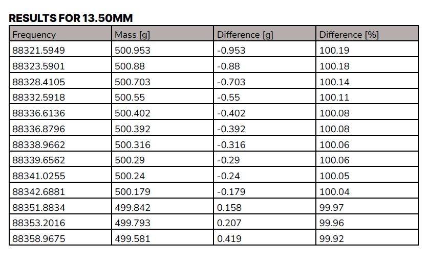
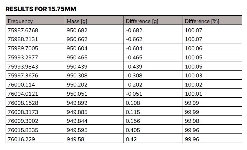
The repeatability is good and sufficiently accurate for the application. This point is a gateway for the development of the frequency-to-weight conversion circuitry.

In this post we looked at the quality of the data, how reproducible the values are and the effect of temperature on the measurement. As the data is non-linear, we investigated two methods to interpolate to get a good mapping between frequency and the applied mass (displacement of the weighing platform).

In the final post we will look at the design of a board used to convert frequency into displacement using a Microchip part which can directly count the input over a gated period.

Part One

Part Two

Part Three

Part Five