


Opinion
Developing A Novel Solution for Measuring Weight - Part 3
Published on 09 Jan, 2024 by Neil
In the last post, we described some basic circuit simulations and initial measurements. In this next chapter, we'll explore the initial measurements and investigate the change in frequency as a function of temperature.
Initial Measurements
Temperature Coefficient
The first characteristic to be investigated is the change in frequency as a function of temperature. The test setup is shown in the diagram below:

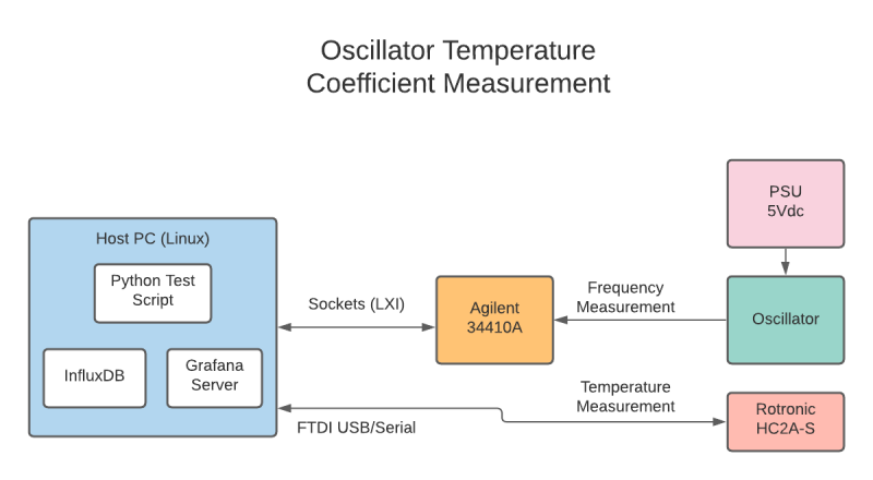
An Agilent 34410A is used to measure the output frequency with a gating time of 1s. The value is read back using a sockets interface accessed via a Python script. At the same time, the temperature is measured using a Rotronic HC2A-S temperature and humidity sensor. The samples are collected every 5s. This record is then written to an InfluxDB time series database for access and analysis at a later time. A typical record takes the following form:
{‘frequency’: 106299.414, ‘humidity’: 37.87, ‘temperature’: 26.48}
{‘frequency’: 106299.299, ‘humidity’: 37.79, ‘temperature’: 26.47}
{‘frequency’: 106299.499, ‘humidity’: 37.84, ‘temperature’: 26.46}
{‘frequency’: 106299.769, ‘humidity’: 37.81, ‘temperature’: 26.46}
{‘frequency’: 106300.014, ‘humidity’: 37.81, ‘temperature’: 26.43}
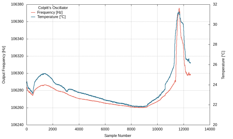
A temperature-controlled environmental chamber was not available, so the oscillator was left running for 24 hours and monitored throughout. The results when viewed using Grafana are below, a close correlation between ambient temperature oscillator output frequency can be observed:

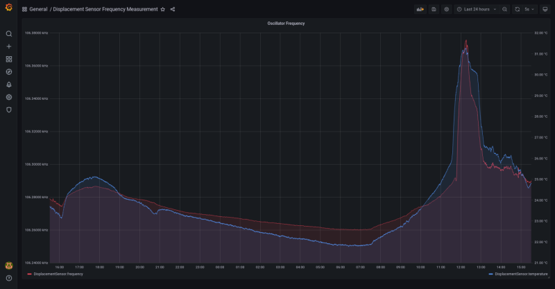
The red trace represents the oscillator output frequency and the blue trace represents the ambient temperature.
Freezer spray was used to cool various components in isolation to try and identify if a single component was particularly temperature-sensitive. The main contributor was the op-amp (frequency rise when cooled), the inductor itself, a frequency rise when cooled, the capacitors have the opposite behaviour, frequency falls when cooled. This makes sense because when the capacitors are cooled, they contract which reduces the distance between the internal plates which will increase their capacitance.
The next challenge is to determine the temperature coefficient over a limited temperature range. This was achieved using Gnuplot.
Tempco Data Analysis
The following command can be used to extract the time series data from InfluxDB.
$ influx -database ‘displacement’ -execute ‘SELECT * FROM DisplacementSensor’-format csvThis can be redirected into a CSV file for plotting. The database name in this example is Displacement.
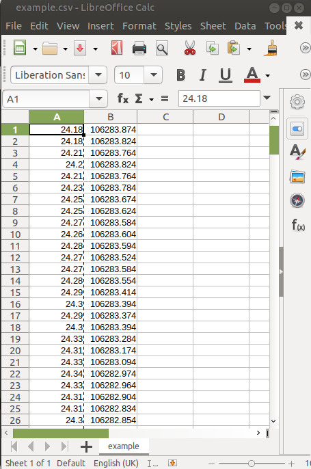
Once Excel or LibreOffice Calc has parsed the CSV file, you will see something like the following:

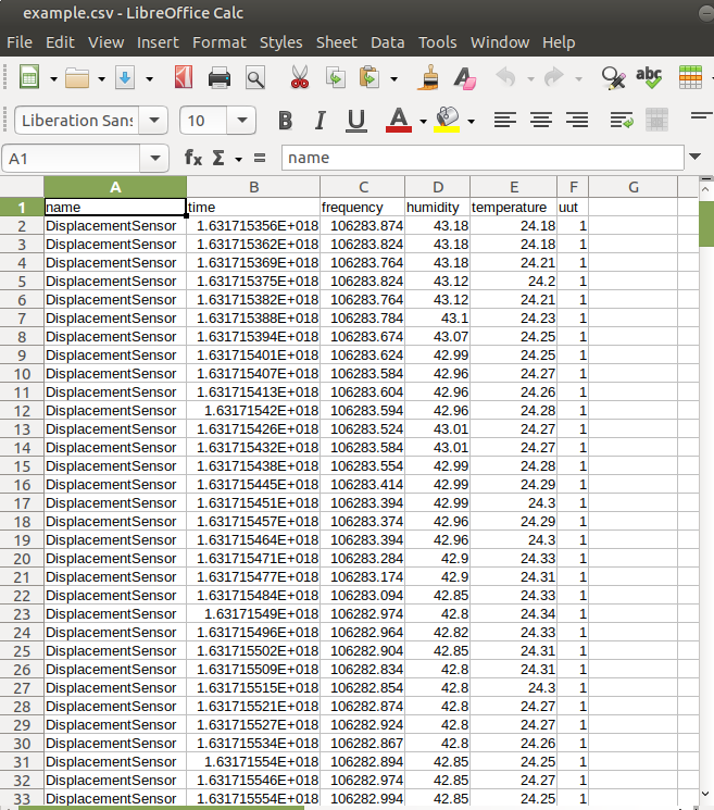
Columns A, B, D and F can be deleted as they are not required for the next steps. Row 1 can also be deleted. Finally, swap the new Columns A and B.

The next step is sorting in ascending order of frequency (column B). Gnuplot is used to plot the frequency as a function of temperature and to determine the gradient of the temperature Coefficient.
Generate Statistics
A simple Gnuplot command will generate many of the statistics (and regression) but does not produce a chart. The command (in file stats.plot for this example) is:
# We are using a CSV file.
set datafile separator ‘,’

# The name of the file containing the data.
stats ‘example.csv’ using 1:2 name “A”

The generated output looks like this:
$ gnuplot stats.plot

* FILE:
Records: 		12438
Out of range: 	0
Invalid: 		0
Column headers: 	0
Blank: 		0
Data Blocks: 	1

* COLUMNS:
Mean:			23.6983 		106276.0816
Std Dev: 		2.0096 		19.4966
Sample StdDev: 	2.0097 		19.4974
Skewness: 		2.0464 		2.8577
Kurtosis: 		7.3013 		12.4566
Avg Dev: 		1.3982 		12.3265
Sum: 			294759.6500 	1.32186e+09
Sum Sq.: 		7.03554e+06 	1.40482e+14

Mean Err.: 		0.0180 		0.1748
Std Dev Err.: 	0.0127 		0.1236
Skewness Err.: 	0.0220 		0.0220
Kurtosis Err.: 	0.0439		 0.0439

Minimum: 		21.7700 [ 0] 	106259.8670 [ 113]
Maximum: 		31.2700 [12437]	106375.7920 [12405]
Quartile: 		22.3500 		106264.2070
Median: 		23.1850 		106270.3670
Quartile:		24.3100 		106280.8730

Linear Model:	y = 9.394 x + 1.061e+05
Slope: 		9.394 +- 0.02173
Intercept: 		1.061e+05 +- 0.5167
Correlation:	r = 0.9683
Sum xy:		3.133e+10
The slope value and residual (r value) are given at the bottom, this will be discussed later. The most interesting points are the range of temperatures (Minimum and Maximum on lines 26 and 27). The data collected covered a range of 21.77°C to 31.27°C. The frequency ranged from 106259.867Hz to 106375.792Hz. This is a span of 115.925Hz over a change of 9.5°C or 115.925 / 9.5 = 12.20Hz/°C
This is an approximation as the slope above shows 9.394Hz/°C.
Viewing the Data
The Gnuplot script is as follows:
(file name freq-vs-temp.plot):
# Set the terminal to generate pngs and the size/
set terminal png size 800,600
# The name of the generated image.
set output “freq-vs-temp-freq-ordered.png”
# We are parsing a CSV file
set datafile separator ‘,’
# Axis labels.
set xlabel “Temperature [°C]”
set ylabel “Output Frequency [Hz]”
# Chart title.
set key title “Colpitts Oscillator”
set key top left Left reverse samplen 1
# Enable the grid
set grid
# Colours for the lines or points.
set style line 1 lt 1 lc rgb ‘#edb120’ # yellow
set style line 2 lt 1 lw 2 lc rgb ‘#e56b5d’ # red
set style line 3 lt 1 lw 1 lc rgb ‘#2c718e’ # blue
# Fit using a linear regression function.
# ‘reference2.csv’ is the file containing the data
# sorted by frequency.
f(x) = m*x + c
fit f(x) ‘reference2.csv’ using 1:2 via m,c
# Display the gradient of the linear regression.
set label sprintf(“m = %3.5g Hz/°C”, m) at screen 0.7,0.3
# Display the intercept (frequency at 0°C).
bfit = sprintf(“c = %6.3f Hz”, c)
set label bfit at screen 0.7,0.26

# Finally plot the data.
plot ‘reference2.csv’ using 1:2 with points ls 3 title ‘Frequency as a
function of temperature’, \
f(x) with lines ls 2 title ‘Line Fit’
This plot file is used in the following way:
$ gnuplot -p freq-vs-temp.plotThere are several interesting features in this chart:

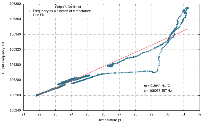
The gradient of the linear regression (m) is 9.3941Hz/°C. At room temperature (22°C) the oscillator is running at 106261.7Hz. As a percentage, this is (9.394/106261.7) * 100 = 0.0088%/°C.
Rising and falling temperatures produce a different slope (notice the two separate curves forming a loop). This could be investigated but is unlikely to be controllable so will be ignored at this stage.
Frequency and Temperature
For completeness, the data collected using InfuxDB is processed using Gnuplot to produce a
frequency versus temperature plot using the following Gnuplot script (file name freq-temp.plot):
# Output configuration and CSV parsing.
set terminal png size 1000,600
set output “freq-temp.png”
set datafile separator ‘,’

# Axis labels
set xlabel “Sample Number”
set ylabel “Output Frequency [Hz]”
20 Green Custard Ltd
set y2label ‘Temperature [°C]’
set key title “Colpitts Oscillator”
set key top left Left reverse samplen 1
set ytics nomirror
set y2tics

# Need to explicitly set the temperature range.
set y2range [20:32]

#set grid

# Colours and styles for the lines.
set style line 1 lt 1 lc rgb ‘#edb120’ # yellow
set style line 2 lt 1 lw 2 lc rgb ‘#e56b5d’ # red
set style line 3 lt 1 lw 2 lc rgb ‘#2c718e’ # blue

# Finally, plot the data.
plot ‘reference3.csv’ using 1:2 axes x1y1 with lines ls 2 title ‘Frequency
[Hz]’,\
‘reference3.csv’ using 1:3 axes x1y2 with lines ls 3 title ‘Temperature
[°C]’
Run as follows:
$ gnuplot freq-temp.plot
The generated chart takes the following form:
Temperature Coefficient Conclusion
The change in frequency of 9.34Hz/°C is not ideal. This needs to be put into the context of the design goals that a change in displacement of 5mm will cover 1kg at a resolution of 10mg. Until the change of frequency per mm of ferrite rod insertion has been determined, it is not possible to know whether the frequency change as a function of temperature makes this approach unworkable.
The frequency does map to the temperature very closely so reliable compensation can be applied. This phase was judged to be a success and the investigation will continue into the linearity of the oscillator with a movable ferrite.
Linearity
The most important characteristic of the displacement sensor is the magnitude of the frequency change as the ferrite is inserted into the inductor. If this value is too low, then the temperature coefficient of the system will make frequency drift a significant part of the measured weight and would be unreliable.
Linearity is the measure of how linear the frequency change is as a function of the insertion depth of the ferrite. This is a reasonably difficult test to perform as the oscillator is very sensitive to changes in inductance and a dedicated fixture needs to be designed and fabricated.
Test Fixture Design
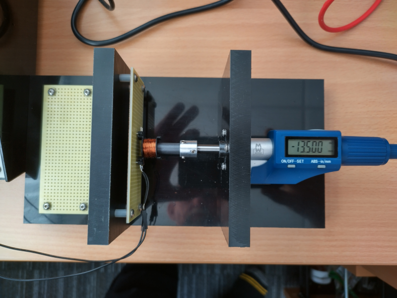
The measurement of frequency as a function of displacement will be made on a bespoke test fixture. The fixture uses a Moore & Wright 312-25D digital micrometre head to accurately extend the ferrite into the coil. The micrometre head has a nominal maximum displacement of 25mm, although ~29.5mm can be achieved.
The micrometre head is mounted in a frame fabricated from 13mm acetal copolymer (a similar material to Delrin, but cheaper). Consideration was given in the design to keep ferrous materials away from the region being measured to try and reduce second-order effects from perturbing the measurements.
The test fixture is shown below:

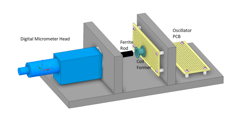
The ferrite rod is mounted axially down the centreline of the fixture. It can only extend along the same axis as the coil and needs to be mounted as concentric as possible with the micrometre head shaft. The diameter of the coil is 8.7mm and the ferrite has a diameter of 8.0mm, which gives a tolerance of 0.35mm. This is tight but possible.
A top view shows the ferrite after it has been extended by 5mm from a zero reference point.

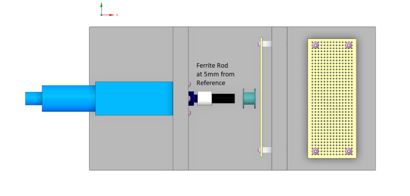
The principle is that an oscillating magnetic field will be emanating from the coil and the influence of the ferrite will not be a step-function, but rather a proportional change in inductance. The test starts with the inductor as far out as possible but with enough travel on the micrometre head to insert the ferrite beyond 50% of the internal coil depth.

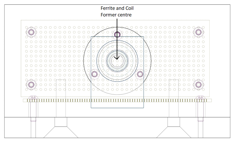
The concentricity was difficult to achieve but with careful design (including mapping the 0.1”
pitch FR4 PCB exactly onto the axial centreline) and fabrication, it was achieved.
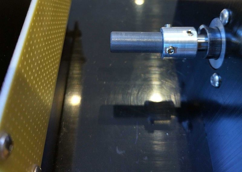
The fixture without the mounted coil is below:

Completed Fixture
The completed fixture is shown below. The oscillator PCB is not populated yet as this current phase needs to decide if further development is justified.

Summary
In this instalment of the blog posts series, the instrumentation of the displacement sensor was described. A series of measurements were made and the test scripts which allowed this were described. Finally, an analysis was performed on the collected data to determine if the displacement sensor was a practicable solution. It was deemed that the results were good enough to continue with the research and the next phase will be described in part four of this series.